Parametric bootstrap for LMLS

A simple parametric bootstrap algorithm for location-scale regression models from the lmls() function.

Usage

boot(m, num_samples = 1000, seed = NULL)

Arguments

m: A location-scale regression model from the lmls() function.
num_samples: The number of bootstrap samples to draw.
seed: Either NULL or an integer that will be used in a call to set.seed() before simulating the response vectors.

Value

An lmls S3 object, see lmls(). The entry boot with the matrices of bootstrap samples is added to the object as a list with the names locationand scale.

Examples

library(lmls)
m <- lmls(y ~ poly(x, 2), ~ x, data = abdom, light = FALSE)
m <- boot(m)
summary(m, type = "boot")
#> 
#> Call:
#> lmls(location = y ~ poly(x, 2), scale = ~x, data = abdom, light = FALSE)
#> 
#> Deviance residuals:
#>      Min.   1st Qu.    Median      Mean   3rd Qu.      Max. 
#> -3.363000 -0.701400 -0.048870 -0.000149  0.623200  4.066000 
#> 
#> Location coefficients (identity link):
#>                Mean    2.5%     50%  97.5%
#> (Intercept)  226.72  225.57  226.72  227.8
#> poly(x, 2)1 2160.67 2130.05 2160.47 2189.2
#> poly(x, 2)2  -99.44 -123.82  -99.80  -73.2
#> 
#> Scale coefficients (log link):
#>                Mean    2.5%     50% 97.5%
#> (Intercept) 1.35344 1.16239 1.35748 1.543
#> x           0.04222 0.03539 0.04218 0.049
#> 
#> Residual degrees of freedom: 605
#> Log-likelihood: -2396.41
#> AIC: 4802.82
#> BIC: 4824.89
#> 
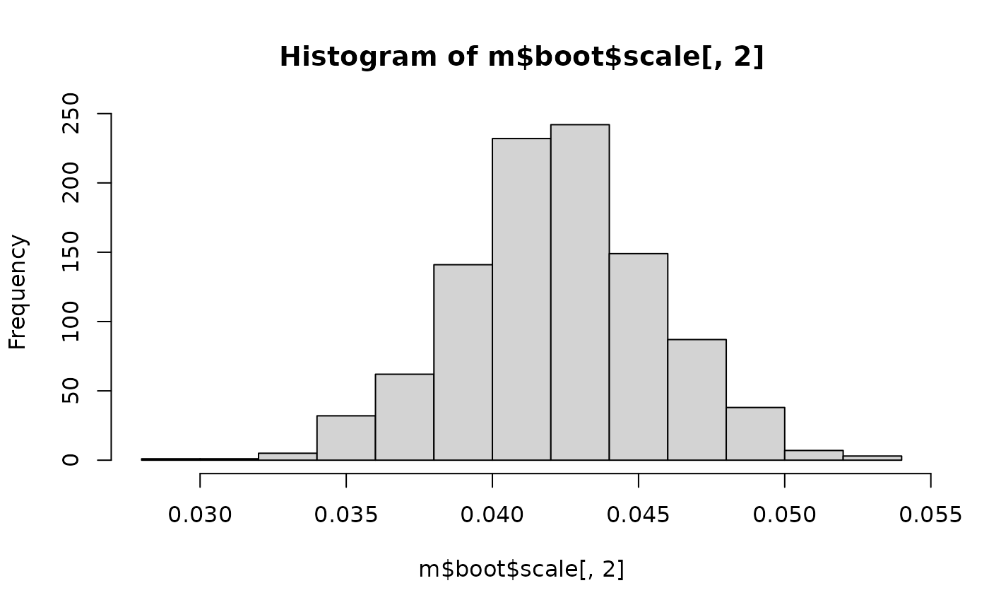
hist(m$boot$scale[, 2])